Monday, 27 July 2015

Subset sum problem -Code in C++

  #include <cmath>  
 #include <cstdio>  
 #include <vector>  
 #include <iostream>  
 #include <algorithm>  
 using namespace std;  
 int main()  
 {  
   int sum=15,arr[10000]={1,2,4,5,9},i,j,n=5;  
   int **a=(int **)malloc((n+1)*sizeof(int*));  
   for(i=0;i<=n;i++)  
     a[i]=(int*)malloc((sum+1)*sizeof(int));  
   for(i=0;i<=n;i++)  
     {  
       for(j=0;j<=sum;j++)  
       {  
       if(j==0)  
        a[i][j]=1;  
       else  
         a[i][j]=0;  
       }  
     }  
   for(i=1;i<=n;i++)  
     {  
       for(j=1;j<=sum;j++)  
       {  
        if(arr[i-1]>j)  
         a[i][j]=a[i-1][j];  
        else  
         a[i][j]=max(a[i-1][j-arr[i-1]],a[i-1][j]);  
       }  
     }  
   for(i=0;i<=n;i++)  
     {  
     cout<<endl;  
     for(j=0;j<=sum;j++)  
       {  
       cout<<a[i][j]<<" ";  
       }  
     }  
     cout<<endl;  
   cout<<((a[i-1][j-1])?"yes":"no");  
   return 0;  
 }  

Sunday, 19 July 2015

Data Structures – TREES- An introduction to trees


Data Structures – TREES

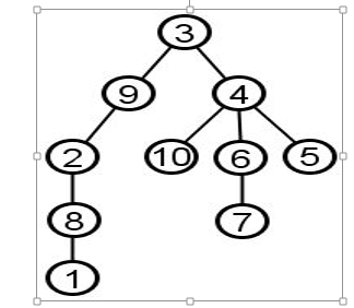
Previously studied Data Structures like Linked Lists or Arrays form the linear structure but trees are the non – linear structures. Trees form the hierarchical form of structure.

Representation of Tree in Computer Science–


If you cannot understand it now, it does not matter. You will understand it in course of time.

Now, most of you must be wondering that WHY TREES??
Trees are important-
1.   For faster search, greater than linked lists but slower than arrays.
2.    For faster insertion and deletion, greater than arrays but slower than linked lists.
3.    To represent the relationship which contains hierarchy naturally like the family or the file system of the computer.                                                                                                 

Terminologies of Tree Data Structure –
1.    Node – Each element in the tree form a node or is called a node.

2.    Edges – The connections connecting the nodes to each other are called edges or  
                    links or branches (for more tree like feeling)
3.    Child Node – The nodes connecting to a node in downward position or the       immediate successors, we can say, are the node’s child node.
In above ex- The node 3, 8 are the child nodes of 5 but node 1, 4 or 7, 10 are not    the child nodes of 5 as they are not immediately connected rather they are termed the grand- children of 5( child of child). This continues like the real family terminology.

4.    Parent Node – The nodes connecting to a node in an upward position (if drawn in the above fashion) or the immediate predecessor of the node are called the parent node of a node. For ex- 3 is the parent of nodes 1 and 3, 8 is the parent node of 7 and 10 but 5 is the grandparent of nodes 1, 4, 7, 10.

5.    Siblings – The nodes which have the same parent are the siblings.

6.    Root Node- The node which have no parent is the root node.


7.    Leaf nodes – Nodes which do not have any children nodes are the leaf nodes or terminal nodes or external nodes.

8.    Internal Nodes – All the nodes which are not the leaf node are the internal node or the interior node including the root itself.

9.    Degree of a node -The number of nodes connected to a node with edges or links form the degree of a node.  In the topmost figure of tree

         Degree(4) = 4 (3 children + 1 parent).

10.          Path- the path is a sequence of nodes and edges connecting a node with a descendant. A path starts from node and ends with another node or leaf. 

Remember –

1.    The path includes all the nodes and edges coming in its way and not just edges.
2.    The path is moving downward and its direction cannot be changed in middle. For ex – there cannot be any path from node 3 to node 6. Also, there cannot be any path from leaf to the root.

11.    Height of a node- The height of a node is the number of edges on the longest downward path between the node and the leaf. The path is always downward so we can remove this redundant word from here.
Each node has height. 3 has height and so does 8 and 7 and etc.
Leaf nodes have no height as there cannot be any path from leaf node to leaf node, so height of leaf node =0.
Keep in mind, it is the longest path so the height of node 5 is the path from node 5 to leaf node 6 and not to any other node like 1, 4 or 7.
          Height of a tree – The height of a tree is the height of the root node itself.
  
 12.    Depth of a node- The depth of a node is the number of edges from the node to the root node.

Depth of root node is 0.

13.    Level of a node- The level of a node is defined as number of connections between the node and the root, or the distance between the node and the root node, with root having level =0. 

    Ex- 5(root node) is at level 0,
    3, 8 at level 1
    1, 4, 7, 10 at level 2

14.    Ancestor of a node – A node A is an ancestor of B if some node A is a parent node    of B or if some child node of A is an ancestor node of B. Stating in simple terms, node A is an ancestor of B if B is child of A or grand-child of A or child of grand – child of A or so on. For ex – 5 is an ancestor of nodes 1, 4, 7, 10.

15.    Descendant of a node – A node A is a descendant of node B if it is child node of B or child of some child of node B. Stating in simple terms, A node A is descendant of node B if B is ancestor of A. For ex- 1, 4, 7 ,10 , 5 ,8 all are descendants of node 5.

  
16.    Forest- the forest, like you may think consist of so many trees, it is same here in the computer science. The forest is made up of n disjoint trees (independent trees) where n >=0.
For ex – if we remove node 5 than node 3 with children 1 and 4 and node 8 with children 7 and 10 form a forest with n=2.

This the forest with two trees (n=2).


Types of Trees –
1 k-ary Trees – the node can have at most k children.
2. Threaded trees – nodes point to their successor or predecessor trough pointers.
3. B- Trees – more than one value can be present in each node.

For more and better visual representations check out our video - https://www.youtube.com/watch?v=FFOTq1RcrBE

Any Queries or updates or any problem in document or the Video that you may want to discuss you can follow our twitter account - https://twitter.com/Logic_Heap
Or you can join our Facebook group - https://www.facebook.com/groups/logicheap/


Sunday, 12 July 2015

0-1 Knapsack Problem - Dynamic Programming

0/1 Knapsack Problem


TYPE:Dynamic programming


Problem- Given some items, pack the knapsack (bag or storage available) to get the maximum total profit. Each item has some weight and some value. Total weight that we can carry is no more than some fixed number W. So we must consider weights of items as well as their value.

Example –

W=9
Vi      
10
40
50
40
40
50
Wi
2
3
4
3
3
4

The Bag may not fill completely.

Solution: We can see that there are various ways through which we can fill our knapsack(bag) while maximizing profit
I.                   Taking weights of 2+3+4=9 with profit of 10+40+50 = 100
II.                 Taking weights of 3+3+2=8 with profit of 40+40+10 = 90
III.              Taking weights of 4+4=8 with profit of 50+50 = 100
IV.              Taking weights of 3+3+3 =9 with profit of 40+40+40 = 120

Now, there are many more cases to consider but they certainly have weight less than8 so we are not considering them, so from here the best solution seems to be the IV. One with bag completely full and profit maximum.

So our main aim is solving the problem such that the profit is maximum with total weight less than or equal to knapsack (cannot be greater).

Now, one can think that why leave the bag empty, why not fill the bag with partial weights like vi=1 etc. So, this thing holds the catch here, in 0/1 Knapsack, we cannot use fractional weights but absolute ones only.

Types of Knapsack Problem-

1.    0/1 Knapsack – the item (Vi) is either used completely or used not at all. We cannot break the item.
2.     Fractional Knapsack- The item can be used in its partial form. We can break the item and use it to fill the bag completely.


Approach for 0/1 Knapsack –

1.             Brute Force Approach
This will take all the possible subsets over the given items list and evaluate the answer.
Let there be n items so there are 2^n possible subsets. We go through all the subsets and find that one subset which is having the maximum value and with total weight less or equal to W(knapsack).

 Accomplished using Divide and Conquer
   We divide the problem into sub problems and solve them and at last stage we combine the solutions of the sub problems to find the final answer.

Algorithm
Knapsack, W = total capacity the person can carry
Array of items, v[0.. n-1] , n = #items
Array of corresponding weights of the items w[0.. n-1]

For every item i, two cases can be considered. Either we take that item or we do not.
Case 1-
If we do not take item i, then we have maximum for weight w over the i-1 items, or
Case 2-
if we include item i, then the value of ith item + recursion over i-1 items with remaining weight (Total weight (W) – weight of ith item(Wi)). The maximum out of these two cases is our answer.

Knapsackbrute (W, v[], w[], n)
if (W==0 || n==0)    // if total weight is zero , then no items can be 
 return 0                // included so 0 , or no item is available then also return 0 */
if( w[n-1] >W)       // if the weight of the nth item is greater than the total weight
return knapsackbrute(W,v,w,n-1)       // available , then only case 1 can be used and we                                                                                     //recurse over the n-1 subproblems 
 else
 return max( knapsackbrute(W,v,w,n-1), v[n-1]+knapsackbrute(W-w[n-1],v, w, n-1)
/* both cases considered */

Time Complexity – O(2^n)
As we are recursing over each possible subset.

Now, the question arises, how can we better it?
Having subproblems which are not independent (subproblems share subsubproblems) divide and conquer is expensive and some method which stores these shared sub problems solution once solved should be used for better time complexity.
2.     The Dynamic Programming Approach is used mostly.
You might wonder why DP and why not Greedy. Let’s just see the latter first.

Why not Greedy??
The greedy approach says that the local optimum is the global optimum. Take the best at each stage and you will end up getting the optimal solution.

  Taking above example –
       Take Wi =4 with maximum Vi = 50, remaining weight = 9-4 =5
        Now, again taking most optimal, Wi = 4 with Vi = 50, remaining weight = 5-4 =1
        No item of Wi =1, so stop.
Our answer from this approach = 50+50 = 100.
But as we have already seen that the best solution is of 120 with weights 3, 3 and 3.
So, the greedy approach won’t work here.


Now to our first question – Why Dynamic Programming?

The answer lies in the very basic properties of DP.

1.     Optimal - Sub Structure- The two cases of divide and conquer strategy above shows this property. we know that if we take some vith item having weight wi then the maximum over remaining weight (W-wi) + weight of vith item gives us the best solution. So the problem jut gets reduced to the again problem having W-wi weight and n-1 items.

2.    Overlapping sub-problems – We already discussed above that if the sub problems are not independent then DP is always a better approach, and we know that for using DP the problem must exhibit this essential property.

Example – W=7 w[]={3, 3,3}  n =3


The highlighted portion shows the overlapping sub problem and hence the DP can be used and will be better.
To reduce time complexity we make a table and store the solutions of the computed sub problems in it, which can be used later when bigger problems come.

The two approaches of DP-

In both the approaches a 2-D table k[n+1][W+1] is used to store the values for n items and total weight = W.

1.      Top Down Approach (Memoization)

Algorithm –

k[n+1][W+1] is declared globally with suitable values of n & W.

memset(k ,-1, sizeof(k[0][0] * (n+1) * (W+1)));  // initialized to -1

intknaptd(int W, int w[] , int v[], int n )
{

   if(W<=0 || n<=0)               // base case
            return 0;
   if (k[n][W]! = -1)// if that value has already been computed
    return k[n][W];
   if(wt[n-1]>W)
   return k[n][W] = knaptd(W, w v,n-1); // total weight in this iteration is less
                                              //than the weight of the nth item so excluding it
    else
    return k[n][W] = max (knaptd(W, w, v,n-1), v[n-1]+knaptd(W-w[n-1], wt , v, n-1) );
}


You may think that this approach is just same as the divide and conquer approach and YES you are correct, but what makes it dynamic and its complexity less than the exponential time is that whatever we are computing through recursion we are storing it in a table for later use.

   Bottom – Up approach


  k[n+1][W+1] is declared globally with suitable values of n & W.


  int knapsack(int W, int w[], int v[] , int n)
      {
            int i , j ; // ith item and jth weight
            memset(k ,0, sizeof(k[0][0] * (n+1) * (W+1)));
          for(i=0; i<=n; i++)// as k is a 2-D matrix so just iterate like that for each item 
            {                                            // and for each item take each weight
            for(j=0; j<=W; j++)
            {
            if(i==0||j==0)// base case
            k[i][j]=0 ;
            else if(j< w[i-1])// total weight in this iteration is less
                                       //than the weight of the  ith item
                     k[i][j] = k[i-1][j];     // not including the ith item
            else
             k[i][j] = max ( k[i-1][j], v[i-1]+k[i-1][j-w[i-1]]);
                                                       // maximum over not                                                                                                                                 //including or including
                                                    // with maximum over i-1 items
            }
            }
        return k[n][W];
     }

Time Complexity- O(nW) , as it stores in a 2-D matrix of size (n+1) *(W+1) and this complexity is much better than the exponential complexity we were getting from brute force approach.

Now before reading any further if you still have doubts over its working or require more visual implementation please refer this link - https://www.youtube.com/watch?v=mZccw_6hOGU

Even after this the doubts persist, be free to ask them over our public group-

And if you are among the lucky ones who have got it , go and solve these problems
3     http://www.spoj.com/problems/LKS/ ( a little trick is required)

You can discuss any of the above problem or any other problem in either our group or on our twitter page –https://twitter.com/Logic_Heap


Implemenation of 0/1 Knapsack  in C++


#include <iostream>
#include<bits/stdc++.h>

using namespace std;
int k[5][60]; // just taken as an example varies as per the problem

// top down using table

intknaptd(int W, int w[] , int v[], int n )
{
    if(W<=0 || n<=0)
    return 0;
    if (k[n][W]!=-1)
    return k[n][W];
    if(wt[n-1]>W)
    return k[n][W] = knaptd(W, w, v,n-1); // total weight in this iteration is less
    // than the weight of the ith item so excluding it
    else
    return k[n][W] = max (knaptd(W, w, v,n-1), v[n-1]+knaptd(W-w[n-1], w , v, n-1) );
}


// Bottom up
int knapsack(int W, int w[], int v[] , int n)
{
    int i , j ; // ith item and jth weight
    
    memset(k ,0, sizeof(k[0][0] * (n+1) * (W+1)));
    
    for(i=0; i<=n; i++)
    {
        for(j=0; j<=W; j++)
        {
            if(i==0||j==0)
            k[i][j]=0 ;
            else if(j< w[i-1])  // total weight in this iteration is less than the weight of the ith item
            k[i][j] = k[i-1][j];  // not including the ith item
            
            else
            k[i][j] = max ( k[i-1][j], v[i-1]+k[i-1][j-w[i-1]]); // maximum over not including or including
            // with maximum over i-1 items
        }
    }
    return k[n][W];
}
int main() {
    int v[] = {60, 100, 120};
    int w[] = {10, 20, 30};
    int W = 50;
    intn = sizeof(v)/sizeof(v[0]);
    printf(“Using Bottom Up Approach”);
    printf("%dn", knapsack(W, w, v, n));
    
    printf(“n Using Top down Approach”);
    memset(k ,-1, sizeof(k[0][0] * (n+1) * (W+1)));
    printf("%dn", knaptd(W, w, v,n));
    return 0;
}


Wednesday, 8 July 2015

Dynamic programming -Maximum sum contiguous sub-array

LOGIC HEAP


ARTICLE CONTRIBUTED BY : Snehil Rastogi ( IIT Roorkee )


NAME: Kadane Algorithm

TYPE: Dynamic Programming

Explanation: Kadane Algorithm is used to find the maximum sum of the contiguous subarray in a given array containing    at least one element.

1.  The naive approach to solve the problem (as discussed in previous video) takes O(n^3) as it considers each sub array then it fixes element in that sub array one by one and then calculates the sum and compare.

2.       Using Divide and Conquer - this approach divides the array into two halves and then recurses over each half and calculates the sum + another module to calculate sum if maximum lies in part of both sub arrays.

 Algorithm -

maxsubarraysum(int a[], int l , int h)
{
    if(l==h)
    return a[l];
    int m = l+(h-l)/2;
 
    /* recurses on left and right subarrays and max sum if subarray crosses the mid point */
 
    maxsum = max(maxsubarraysum(a,l,m), maxsubarraysum(a,m+1,h), maxinboth(a,l,m,h));

     /* data type of maxsum(here int ) same as type of array */
 
    return maxsum;
}

maxinboth(int a[], int l , int m , int h)
{
    int sum=0;
    int lsum = INT_MIN;
    for(i=m;i>=l;i--)
    {
        sum+=a[i];
        if(lsum<sum)
        lsum = sum;
    }
 
    int rsum = INT_MIN;
    sum=0;
    for(i=m+1; i<=h;i++)
    {
        if(rsum<sum)
        rsum=sum;
    }
    return lsum+rsum;
}

Time Complexity = 2T(n/2)+O(n) = O(nlogn)


3.       Dynamic Programming Approach - The array is traversed only once.

Two variables currmax (hold the current maximum for each element of the array) and totalmax ( holding the   total maximum encountered so far , at the end it holds the answer to the maximum sum found)
        
Apart from these the variables index, maxsindex ( holding the starting index of the subarray whose sum is largest),    maxeindex (holding the ending index of the subarray whose sum is largest) holds the values for the indices.

The algorithm is –

Maxsubarraysum(int a[], int n)   // the entered array and its size
currmax = a[0], toalmax=a[0];
index =0, maxsindex =0, maxeindex =0;    // initially the starting value and starting index

// now traverse the remaining array

for( i=1 to n)

/*check  maximum among current a[i] and  current max + a[i]  – this step holds its importance if negative numbers are present  in the array , if only positive numbers are present in the array then the comparison
currmax +=a[i]
if(currmax < 0)  currmax=0;
would suffice
but with negative numbers present this won’t work(obviously) */

if( a[i] > currmax+a[i])
currmax = a[i];
index =i ;         //for holding the index intermediately element wise

else
currmax = currmax+a[i];

// now compare with overall total encountered so far

If(totalmax < currmax)
totalmax = currmax;
maxsindex = index;
maxeindex = i;

print (totalmax , maxsindex , maxeindex)
Time Complexity – as we are traversing the array only once so O(n) , much less then the naïve approach and better then the divide and conquer strategy discussed .

Uses & Applications –
This is a very important algorithm and quite easy to understand. It is often asked in the interview questions.

Extensions –
1.       Finding maximum sum in square sub matrix from a 2-D array.
2.       Finding maximum sum in circular sub array
3.       Finding maximum product  in a sub array (the approach is exactly same with just one simple change)


Problems to try on –


These are some of the simplest and direct applications of the Kadane algorithm. Do go and try these for the better understanding of the algorithm. 


KADANE'S Algorithm for minimum/ maximum sum on a contiguous subarray having both positive and negative values


 #include <iostream>
#include<bits/stdc++.h>
using namespace std;
void maxSubArraySum(int a[], int n)
{
    int i;
    int currmax = a[0];                 //holding the maximum for each index
    int  totalmax = a[0];               //holding the overall maximum(answer) for the specific sub array
  
    // starting and ending indices of the subarray whose sum is maximum
  
    int index =0, maxsindex=0,maxeindex=0;
    for(i=1 ; i<n; i++)
    {
        // as negative numbers are also present in the array so comparison with a[i] is essential
        if(a[i] >= currmax + a[i])
        {
          
            currmax = a[i];
            index=i;
        }
        else
        currmax = currmax + a[i];
      
        if(currmax >= totalmax)
        {
            totalmax = currmax;
            maxsindex = index;                         // update the indices
            maxeindex=i;
        }
    }
    printf("%dt%dt%dn",totalmax,maxsindex,maxeindex);
  
}

/* same as maxSubArraySum() , only comparison opeartor reversed as we are now checking for minimum in a contiguous sub array
*/
void minSubArraySum(int a[], int n)
{
  
    int currmin=a[0], totalmin=a[0],index=0, minsindex=0, mineindex=0, i;
    for(i=1; i<n; i++)
    {
        if(a[i]<=currmin+a[i])
        {
            currmin=a[i];
            index=i;
        }
        else
        currmin= currmin+a[i];
      
        if(totalmin>currmin)
        {
            totalmin=currmin;
            minsindex=index;
            mineindex=i;
        }
    }
    printf("%dt%dt%dn",totalmin,minsindex,mineindex);
}


int main() {
  
    int a[] =  {6, 3, 10, 0, -12, 3 , -11, -10};
    int n = sizeof(a)/sizeof(a[0]);
  
    maxSubArraySum(a, n);
    minSubArraySum(a,n);
    return 0;
}